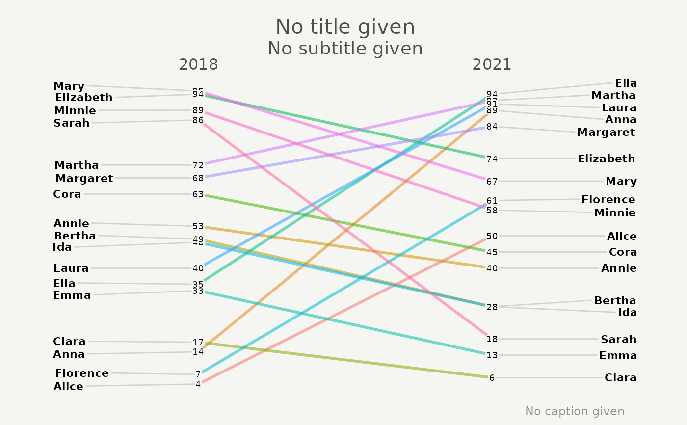
Slope graph for ggplot2 — ggslope • HohgantR

Creates a slope graph ideal to use when computing changes in one or more indicators between waves of a survey or other time series data with a low number of periods.

Usage

ggslope(
  data,
  x,
  y,
  group,
  DataLabel = NULL,
  title = "No title given",
  subtitle = "No subtitle given",
  caption = "No caption given",
  LineThickness = 1,
  LineColor = "ByGroup",
  DataTextSize = 2.5,
  DataTextColor = "black",
  DataLabelPadding = 0.05,
  DataLabelLineSize = 0,
  DataLabelFillColor = "#f5f5f2",
  WiderLabels = FALSE,
  ReverseYAxis = FALSE,
  ReverseXAxis = FALSE,
  RemoveMissing = TRUE
)

Source

Adapted and updated from this great package.

Arguments

data: Data frame containing the data in a long form. Required input.
x: The variable on the x axis, usually time, survey wave, etc. Required input.
y: The variable on the y axis, usually an indicator such as poverty and inequality measures. Required input.
group: Grouping variable showing various levels of the indicator.
DataLabel: Data label
title: Plot title
subtitle: Plot subtitle
caption: Plot caption
LineThickness: Line width
LineColor: Line color
DataTextSize: Text size of the data point value.
DataTextColor: Text color of the data point value.
DataLabelPadding: Text padding of the label of each level.
DataLabelLineSize: Text label line size.
DataLabelFillColor: Text label fill color.
WiderLabels: Set wider labels? False by default.
ReverseYAxis: Revert Y axis? False by default.
ReverseXAxis: Revert X axis? False by default.
RemoveMissing: Remove missing values? True by default.

Value

A pretty slope graph.

Examples

HohgantR::indicators_long |>
dplyr::filter(indicator == "Indicator") |>
ggslope(year, value, unit)